Chapter 10: Music, Number and Nature

Topics: Connecting nature, music and number, Pythagorean theorem, music from math curves, sin() and cos() functions, the Python math library, visualizing oscillations, the harmonograph, sonifying oscillations, Kepler’s harmony of the world revisited.

In the previous chapters, we studied essential building blocks of music and computer science. We now know enough about music and programming to return to the themes introduced in Chapter 1. In this chapter, we will deepen our exploration into the connections between music, number, and nature, and introduce you to ideas that will hopefully inspire and guide you in your own personal journey into music and programming. More information is provided in the reference textbook.

Here is code from this chapter:

• Making music from math curves
• Simulating a lateral harmonograph
• Simulating a rotary harmonograph
• Non-integer ratios
• Kepler’s Harmony of the World, No. 2

---

Making music from math curves

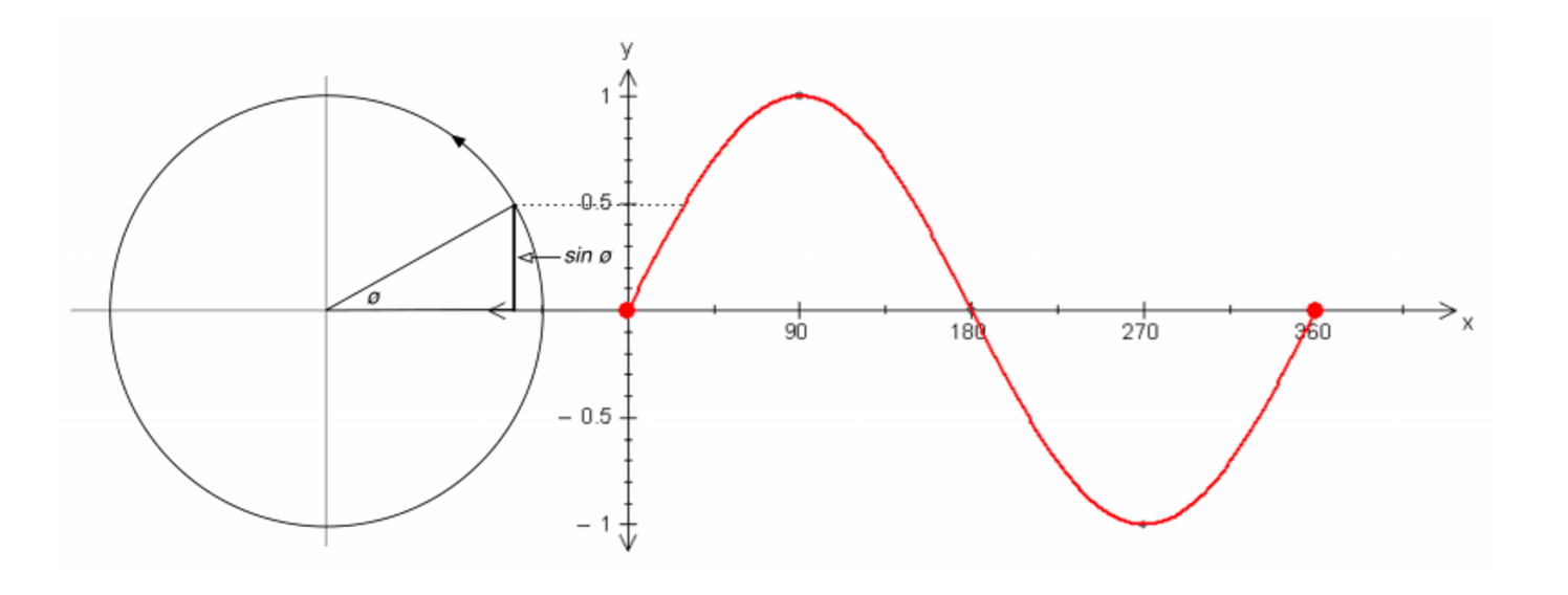
A simple mathematical function is the sine. It describes a smooth repetitive oscillation (i.e., a wave), as shown below:

Two complementary views of the sine function: (left) as the rise of a point traversing a unit circle, and (right) as the wave graph been drawn by that point (imagine the circle moving to the right, while the point is rotating)

The code sample below (Ch. 10, p. 321) demonstrates how to create a simple melodic contour using the Python sin() function. It also creates a visual

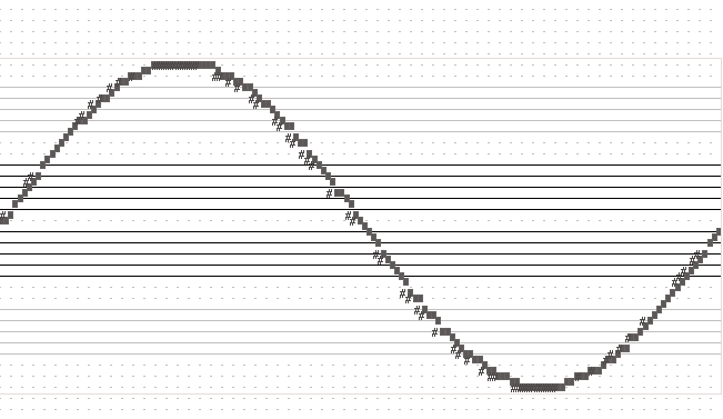
It also creates a visual pianoroll, which traces the sine wave oscillation:

Melodic contour from a sine wave

Here is the program:

# sineMelody.py
#
# This program demonstrates how to create a melody from a sine wave.
# It maps the sine function to a melodic (i.e., pitch) contour.
#

from music import *
from math import *

phr = Phrase()
density = 25.0                 # higher for more notes in sine curve
cycle = int(2 * pi * density)  # steps to traverse a complete cycle

# create one cycle of the sine curve at given density
for i in range(cycle):
   value = sin(i / density)    # calculate the next sine value
   pitch = mapValue(value, -1.0, 1.0, C2, C8)   # map to range C2-C8
   note = Note(pitch, TN)
   phr.addNote(note)
# now, all the notes have been created

View.pianoRoll(phr)  # so view them
Play.midi(phr)       # and play them

It plays this sound:

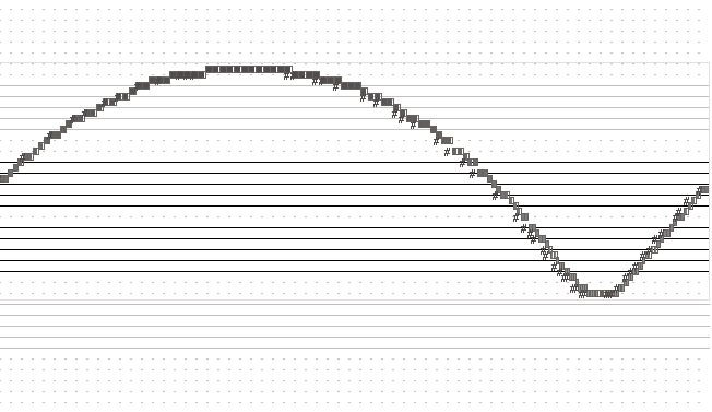
Next we connect additional musical parameters to the sine function, namely, note duration, dynamic, and panning. The piano roll generated by the updated program is shown below. Notice the distortion in the sine wave graph. Why does that happen?

Melodic contour from sine wave also mapped to duration of notes

Here is the code:

# sineMelodyPlus.py
#
# This program demonstrates how to create a melody from a sine wave.
# It maps the sine function to several musical parameters, i.e.,
# pitch contour, duration, dynamics (volume), and panning.
#

from music import *
from math import *

sineMelodyPhrase = Phrase()
density = 25.0                 # higher for more notes in sine curve
cycle = int(2 * pi * density)  # steps to traverse a complete cycle

# create one cycle of the sine curve at given density
for i in range(cycle):
   value = sin(i / density)    # calculate the next sine value
   pitch = mapValue(value, -1.0, 1.0, C2, C8)   # map to range C2-C8
   #duration = TN
   duration  = mapValue(value, -1.0, 1.0, TN, SN)   # map to TN-SN
   dynamic = mapValue(value, -1.0, 1.0, PIANISSIMO, FORTISSIMO)
   panning = mapValue(value, -1.0, 1.0, PAN_LEFT, PAN_RIGHT)

   note = Note(pitch, duration, dynamic, panning)
   sineMelodyPhrase.addNote(note)

View.pianoRoll(sineMelodyPhrase)
Play.midi(sineMelodyPhrase)

It plays this sound:

---

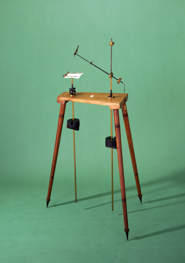
The Harmonograph

The harmonograph is used to study harmonic oscillations. It has a pen and two pendula moving in orthogonal directions. As the pendula move, the pen draws on paper.

There are two versions, lateral and rotary.

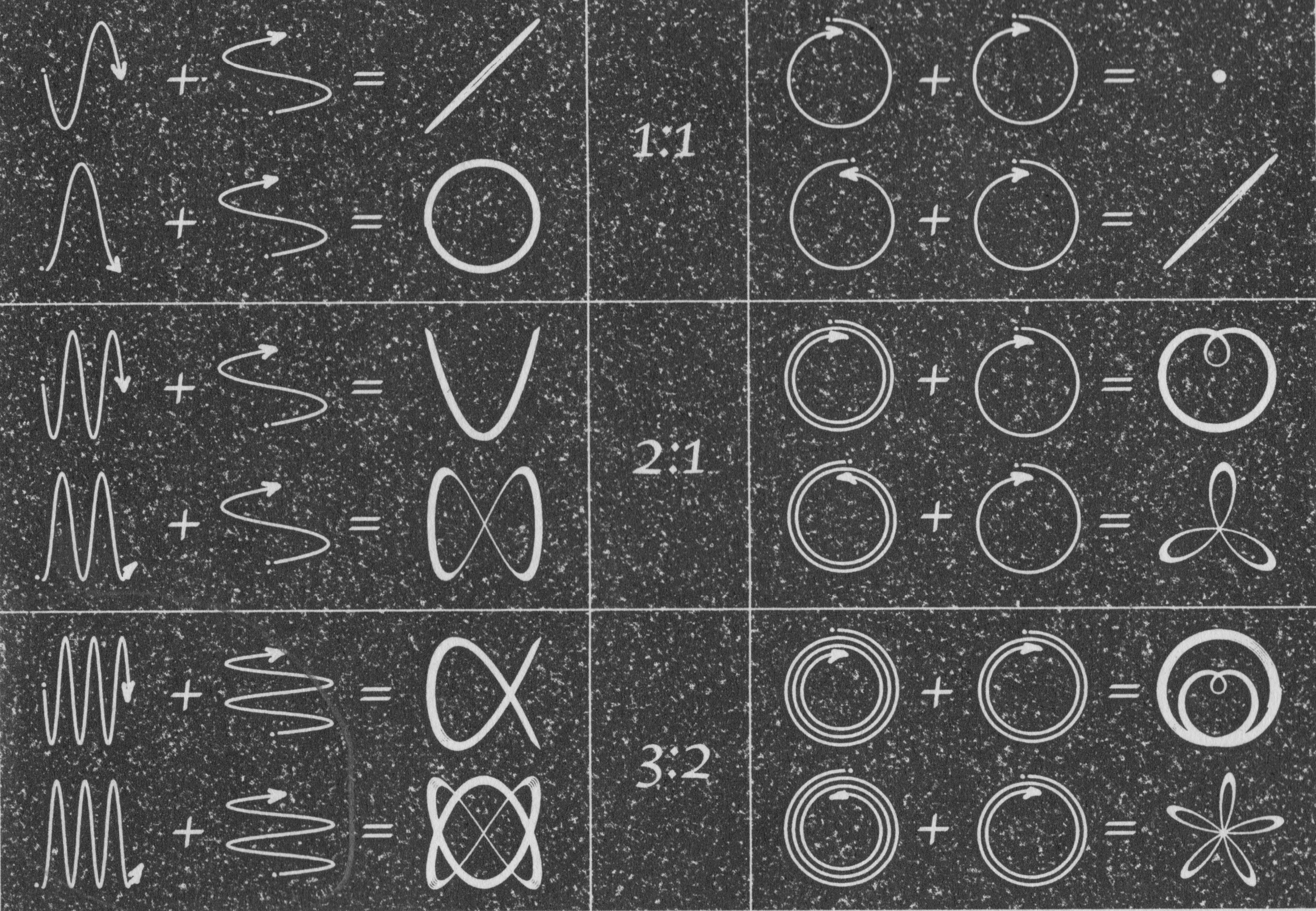
Harmonographs are used to visualize music intervals (harmonic ratios). For example, here are shapes generated from different harmonic ratios (i.e., 1:1, 2:1, and 3:2). Lateral harmonograph on the left; rotary harmonograph on the right.

Using lateral harmonograph (left) and rotational harmonograph (right) to draw shapes for different ratios (e.g., 1:1, 2:1, etc.) (Ashton, 2003, p. 19)

Simulating a lateral harmonograph

A lateral harmonograph has a pen attached to two pendula moving in orthogonal directions (see below). As pendula move, the pen draws on paper.

A lateral harmonograph

The code sample below (Ch. 10, p. 328) simulates a lateral harmonograph. We may adjust:

• Length of pendula — this affects frequency of oscillation. By combining different frequency ratios (e.g., 2:3), we get different shapes (as shown above).
• Phase of pendula, relative to one another. This can be same, or reverse.

Here is the code:

# harmonographLateral.py
#
# Demonstrates how to create a lateral (2-pendulum) harmonograph
# in Python.
#
# See Ashton, A. (2003), Harmonograph: A Visual Guide to the
# Mathematics of Music, Wooden Books, p.19.
#

from gui import *
from math import *

d = Display("Lateral Harmonograph", 250, 250)
centerX = d.getWidth() / 2    # find center of display
centerY = d.getHeight() / 2

# harmonograph parameters
freq1 = 2   # holds frequency of first pendulum
freq2 = 3   # holds frequency of second pendulum
ampl  = 50  # the distance each pendulum swings

density = 50                   # higher for more detail
cycle = int(2 * pi * density)  # steps to traverse a complete cycle
times = 6                      # how many cycles to run

# display harmonograph ratio setting
d.drawText("Ratio " + str(freq1) + ":" + str(freq2), 95, 20)

# go around the unit circle as many times requested
for i in range(cycle * times):

   # get angular position on unit circle (divide by a float
   # for more accuracy)
   rotation = i / float(density)

   # get x and y coordinates (run and rise)
   x = sin( rotation * freq1 ) * ampl   # get run (same phase)
   #x = cos( rotation * freq1 ) * ampl   # get run (opposite phase)
   y = sin( rotation * freq2 ) * ampl   # get rise

   # convert to display coordinates (move display origin to center,
   # from top-left)
   x = x + centerX
   y = y + centerY

   # draw this point (pixel coordinates are int)
   d.drawPoint( int(x), int(y) )

It generates this shape:

---

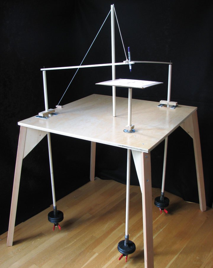
Simulating a rotary harmonograph

A rotary harmonograph has a pen attached to two pendulums moving in orthogonal directions. As the pendulums move, the pen draws on paper. The paper is placed on a third pendulum on a rotary bearing (i.e., gimbals). This provides another oscillation to the system.

A rotary harmonograph

The code sample below (Ch. 10, p. 330) simulates a rotary harmonograph. We may adjust:

• Length of pendula — this affects frequency of oscillation. By combining different frequency ratios (e.g., 2:3), we get different shapes (as shown above).
• Phase of pendula, relative to one another. This can be same, or reverse.

This program can also dampen oscillations (via friction). To do so, uncomment the last two statements. This introduces more interesting shapes.

Here is the code:

# harmonographRotary.py
#
# Demonstrates how to create a rotary (3-pendulum) harmonograph
# in Python.
#
# Here, the position of the pen is determined by two pendula,
# and is modeled by either (sin, sin) or (cos, sin).
# The third pendulum has its own sin() and cos() to model the second
# circle.
#
# See Ashton, A. (2003), Harmonograph: A Visual Guide to the
# Mathematics of Music, Wooden Books, p.19.
#

from gui import *
from math import *

d = Display("Rotary Harmonograph", 250, 250)
centerX = d.getWidth() / 2    # find center of display
centerY = d.getHeight() / 2

# harmonograph parameters
freq1 = 2     # holds frequency of first pendulum
freq2 = 3     # holds frequency of second pendulum
ampl1 = 40    # holds swing of movement for pair of pendulums
              # (radius of first circle)

ampl2 = ampl1 # holds swing of movement for third pendulum
              # (radius of second circle)

#friction = 0.0003   # how much energy is lost per iteration

density = 50                  # higher for more detail
cycle = int(2 * pi * density)  # steps to traverse a complete cycle
times = 1                      # how many cycles to run

# display harmonograph ratio setting
d.drawText("Freq Ratio " + str(freq1) + ":" + str(freq2), 80, 10)

# go around the unit circle as many times requested
for i in range(cycle * times):

   # get angular position on unit circle (divide by a float
   # for more accuracy)
   rotation = i / float(density)

   # get x and y coordinates (run and rise)
   x1 = sin( rotation * freq1 ) * ampl1  # get run (same phase)
   y1 = cos( rotation * freq1 ) * ampl1   # get rise
   #x1 = cos( rotation * freq1 ) * ampl1  # get run (opposite phase)
   #y1 = sin( rotation * freq1 ) * ampl1   # get rise

   x2 = sin( rotation * freq2) * ampl2   # get run (second pendulum)
   y2 = cos( rotation * freq2) * ampl2   # get rise

   # combine the two oscillations
   x = (x1 - x2)
   y = (y1 - y2)

   # convert to display coordinates (move display origin to center,
   # from top-left)
   x = x + centerX
   y = y + centerY

   # draw this point (pixel coordinates are int)
   d.drawPoint( int(x), int(y) )

   # loss some energy due to friction
#   ampl1 = ampl1 * (1 - friction)
#   ampl2 = ampl2 * (1 - friction)

It generates the following shape.

NOTE: This is also the shape drawn by planet Venus on Earth’s sky (Venus rotates around the Sun about 13 times for every 8 Earth rotations). This observation (and trying to explain it) may have been the beginning of science (math, astronomy, physics) and music (scales) by the ancients. The above program distills all those centuries of knowledge development, in just a few lines.

---

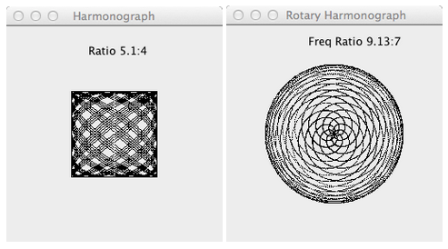
Non-integer ratios

Non-integer ratios correspond to musical intervals that are not harmonious (and not pleasing to the ear).

Such ratios generate chaotic paths as traced by the harmonograph. When exploring, increase the value of variable times to allow the pen to trace orbits over several cycles – to better see the behavior that emerges.

For example, here are two shapes generated by non-harmonic ratios (5.4 : 4, and 9.13 : 7).

(Left) Lateral harmonograph – 5.01 : 4 ratio, same phase, 6 times. (Right) Rotary harmonograph – 9.13 : 7 ratio, same phase, 6 times.

Certain ratios result in paths that will never converge (i.e., never re-trace the same path).

NOTE: The faster a ratio begins to retrace the same path, the more harmonious (consonant) it sounds to our ear. See Legname’s Theory on Density of Intervals (Legname 1998).

---

Kepler’s Harmony of the World, No. 2

Here is another sonification of the planets, influenced by the harmonograph above (also see chapter 7).

This code sample (Ch. 10, p. 334) sonifies planetary velocities. It uses sines and cosines to simulate movement (sound spatialization).

Here is the code:

# harmonicesMundiRevisisted.py
#
# Sonify mean planetary velocities in the solar system.
#

from music import *
from math import *
from random import *

# Create a list of planet mean orbital velocities
# Mercury, Venus, Earth, Mars, Ceres, Jupiter, Saturn, Uranus,
# Neptune. (Ceres is included in place of the 5th missing planet
# as per Bode's law).
planetVelocities = [47.89, 35.03, 29.79, 24.13, 17.882, 13.06, 9.64,
                    6.81, 5.43]
numNotes     = 100       # number of notes generated per planet
durations    = [SN, QN]  # a choice of durations
instrument   = EPIANO    # instrument to use
speedFactor  = 0.01      # decrease for slower sound oscillations

score = Score(60.0)      # holds planetary sonification

# get minimum and maximum velocities:
minVelocity = min(planetVelocities)
maxVelocity = max(planetVelocities)

# define a function to create one planet's notes - returns a Part
def sonifyPlanet(numNotes, planetIndex, durations, planetVelocities):
   """Returns a part with a sonification of a planet's velocity."""

   part = Part(EPIANO, planetIndex)   # use planet index for channel
   phr = Phrase(0.0)

   planetVelocity = planetVelocities[planetIndex]   # get velocity

   # create all the notes by tracing the oscillation generated using
   # the planetary velocities
   for i in range(numNotes):

      # pitch is constant
      pitch = mapScale(planetVelocity, minVelocity, maxVelocity,
                       C3, C6, MIXOLYDIAN_SCALE, C4)

      # panning and dynamic oscillate based on planetary velocity
      pan = mapValue(sin(i * planetVelocity * speedFactor * 2),
                     -1.0, 1.0, PAN_LEFT, PAN_RIGHT)
      dyn = mapValue(cos(i * planetVelocity * speedFactor * 3),
                     -1.0, 1.0, 40, 127)

      # create the note and add it the the phrase
      n = Note(pitch, choice(durations), dyn, pan)
      phr.addNote(n)

   # now, all notes have been created

   part.addPhrase(phr)  # add phrase to part
   return part          # and return it

# iterate over all plants
for i in range( len(planetVelocities) ):
   part = sonifyPlanet(numNotes, i, durations, planetVelocities)
   score.addPart(part)

View.sketch(score)
Play.midi(score)

It plays this sound:

(use stereo headphones to hear movement – front-to-back, and left-to-right)

For more details, see this book.